Overview
ForestMaps – Modeling Utilization of Forests
This project seeks to compute utilization information for public spaces, in particular forests: which parts of the forest are used by how many people.
We developed a sound model for computing this information from publicly available data such as road maps and population counts. This website is an interactive web application, that visualizes our result as a heat-map layer on top of OpenStreetMap data in the widget above. The colors encode the utilization of the underlying ways. Areas with more intesive colors are more frequented that those blue or no color. Use the mouse to navigate and zoom in the map. You can switch between different datasets using the drop-down on the top right corner of the page.
The desired utilization information of our model is computed using efficient algorithms, which are presented in the Components section of this page. We provide an experimental evaluation of different variations of our algorithms, which we compare with respect to efficiency and quality in the Results section. Our source code and the data sets used to conduct the experiments can be accessed in the Downloads section. The functioning of this webapp is explained in About.
Motivation – The Role of the Forests
Nowadays mankind uses the forests in its surroundings not only for leisure activities and lumbering. The woods also fulfill an important part of keeping the worlds ecosystem in balance and must therefore be conserved. These three major functions conflict each other. Ongoing logging naturally inhibits the ability of the forests to provide for a basis of biodiversity. Also steady presence of humans scares off animals and takes a heavy toll on nature's health.
Governments aim to divide the forestal areas into parts fulfilling the functions explained above. A model of forest utilization serves as a basis for this regulation. Unfortunately, statistics about people's activity inside the forest are hard to obtain. Other than in road networks, the frequency along hiking trails is too low and varies strongly between sunny and rainy days, so counting of visitors using humans or computers does not pay off.
Components
Pipeline
The image below summarizes the pipeline of algorithms we use to compute the utilization distribution. We extract road graphs and the borders of forest areas from OpenStreetMaps data (note that the approach can easily be extended to ESRI shape files, for example). We then compute positions where roads or paths enter the woods. For each such place we compute the number of peoples who are likely to use it to enter the forest based on the number of people living in the surrounding. The latter information is computed from OpenStreetMaps and ontologies like Wikipedia or GeoNames. Next, we determine practical (round) trips between forest entries. Finally, the intermediate results from the beforehand steps are joined to a utilization map of the forest.
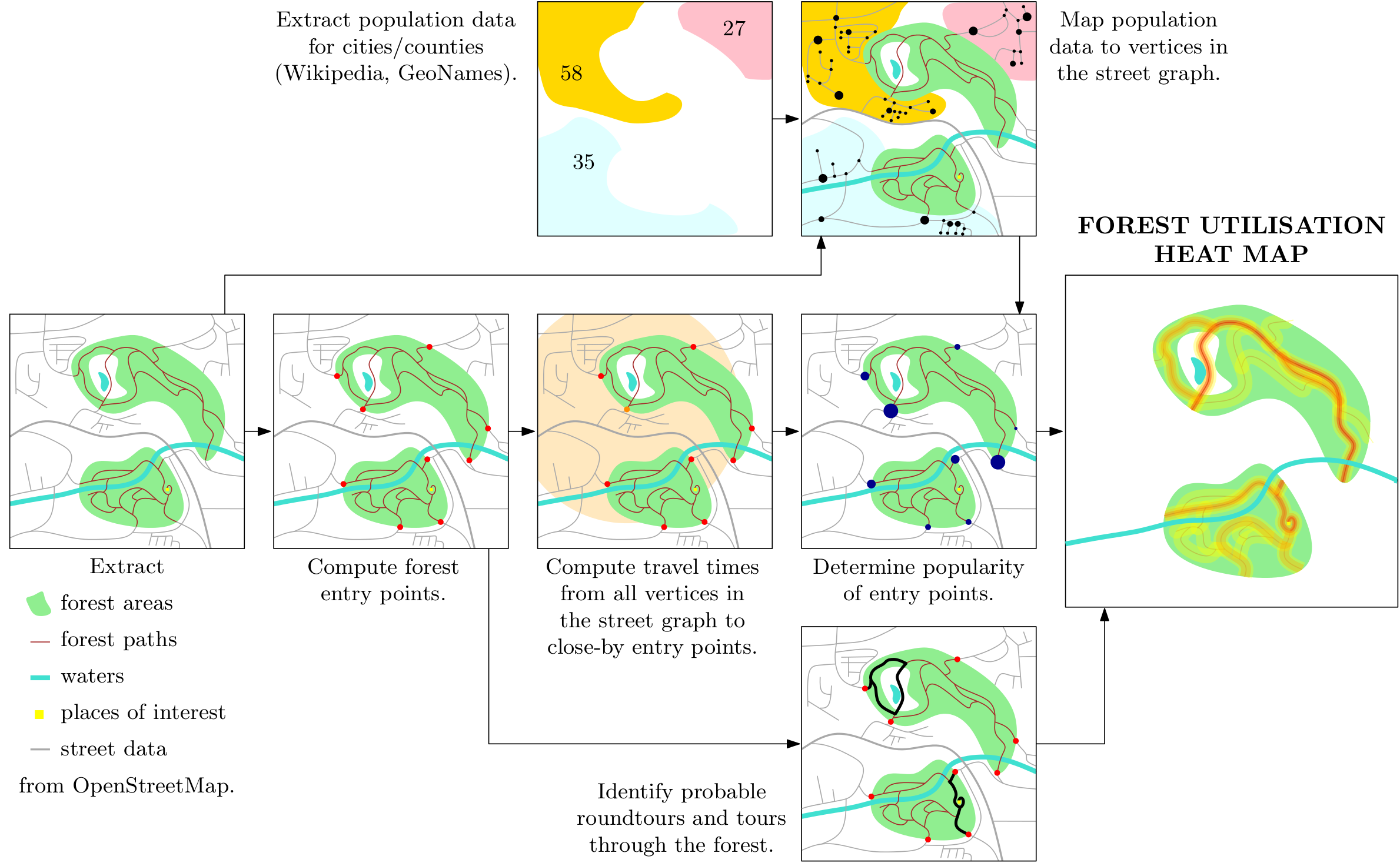
Data extraction
OpenStreetMap.org provides geographic information described by XML-markup for nodes (geographic locations with latitude and longitude), polygonal paths (so called ``ways'', referencing previously defined nodes) and compositions thereof (``relations'', referencing sets of nodes, ways or relations). Each entity can have several attached tags, which are tuples of the form key:value. We parse all nodes, ways, and relations from the relevant OSM files and translate relations and ways to sequences of coordinates. We then build the road network from ways with a highway:* tag. We generate the forest areas from entities with tags landuse:forest and natural:wood. Polygons with tag boundary:administrative are retrieved as boundaries of municipalities. Furthermore, we select nodes whose tags match certain combinations of tags as points of interest (POIs). For example, places with the tags man_made:tower and tourism:viewpoint are considered as POI.
Population data for countries and cities can be obtained from Wikipedia's infoboxes. For example, see Freiburg.
Forest entry point detection
We have to find all edges from the road graph that intersect one of the forest polygons. We check for each node of the network if it falls inside a forest polygon or not using a canvas approach: To handle the large numbers of nodes for which the membership test has to be done, we rasterize the polygon to a bit array. Consider this as image, where the forest areas are painted in green and the remaining parts are white. Using this classification, we iterate over all nodes in the graph and check for nodes outside the forest if they have an adjacent edge towards a node inside the forest.
Population distribution estimation
We need to know the population distribution in the area surrounding the forests. Specifically, we need an estimate of the number of people that live near each street segment of the road network. We assume that the population density and the density of local streets coincide. This allows to use a Voronoi-diagram of the road network to assign a population share to each street.
Popularity of forest entries
We use Dijkstra's famous algorithm to compute the forest entries reachable below some timelimit (say 1 hour) for every place on the map. Depening on the previously computed population of the streets, on the number of available forests and their distance every forest entry the popularity of each forest entry can be calculated.
Attractiveness of forest trails
We implemented two approaches for computing the attractiveness of trails in the forest. The first one can be considered as flooding the entry points' popularity into the nearby forest. The second, more elaborate approach computes the attractiveness by taking into account every way segment's position in relation to shortest paths paths between entry points. The Result part of this website compares the results of these two methods.
Putting things together
Combining the entry points' popularities with attractiveness of single edges in the forest, we get a utilization estimate for every part of the forest. Painting these values as an overlay to the original map results in a heatmap, like the one you have seen above. Our model gives pretty good estimates for the data sets we have evaluated so far. You can find some details in the Results section.
Results
This page shows the results of an experimental evaluation of our model on different OSM data sets.
Computation time
The table below shows the measured the running time for each step of our pipeline excluding the data extraction from OSM.
| Graph | Runtime (in seconds) | ||||
|---|---|---|---|---|---|
| population mapping | entry point extraction | entry point popularity | path attractiveness | total | |
| Saarland | 0.01 | 1.92 | 63.53 | 40.65 | 2min |
| Switzerland | 0.38 | 11.95 | 51.20 | 211.34 | 5min |
| Baden-Württemberg | 0.43 | 20.78 | 584.65 | 1223.43 | 31min |
| Austria | 0.79 | 24.15 | 56.78 | 912.55 | 17min |
| Germany | 2.86 | 181.25 | 512.29 | 6958.33 | 135min |
We observed that the fraction of time spent on the population mapping is negligible. It is just a few seconds even for our largest data set (Germany). This is easy to understand, since the computation of the street Voronoi-diagram requires only a single sweep over all edges. The fraction of time spent on the FEP extraction is also relative small. This is due the efficient rasterization approach. The two remaining steps, the computation of the FEP popularity values and of the forest path attractiveness values are the most time-consuming of our whole pipeline. This is because both steps require a large number of Dijkstra computations. The simple flooding approach is about 40 times faster than the via-edge approach.
Quality of the population distribution estimation
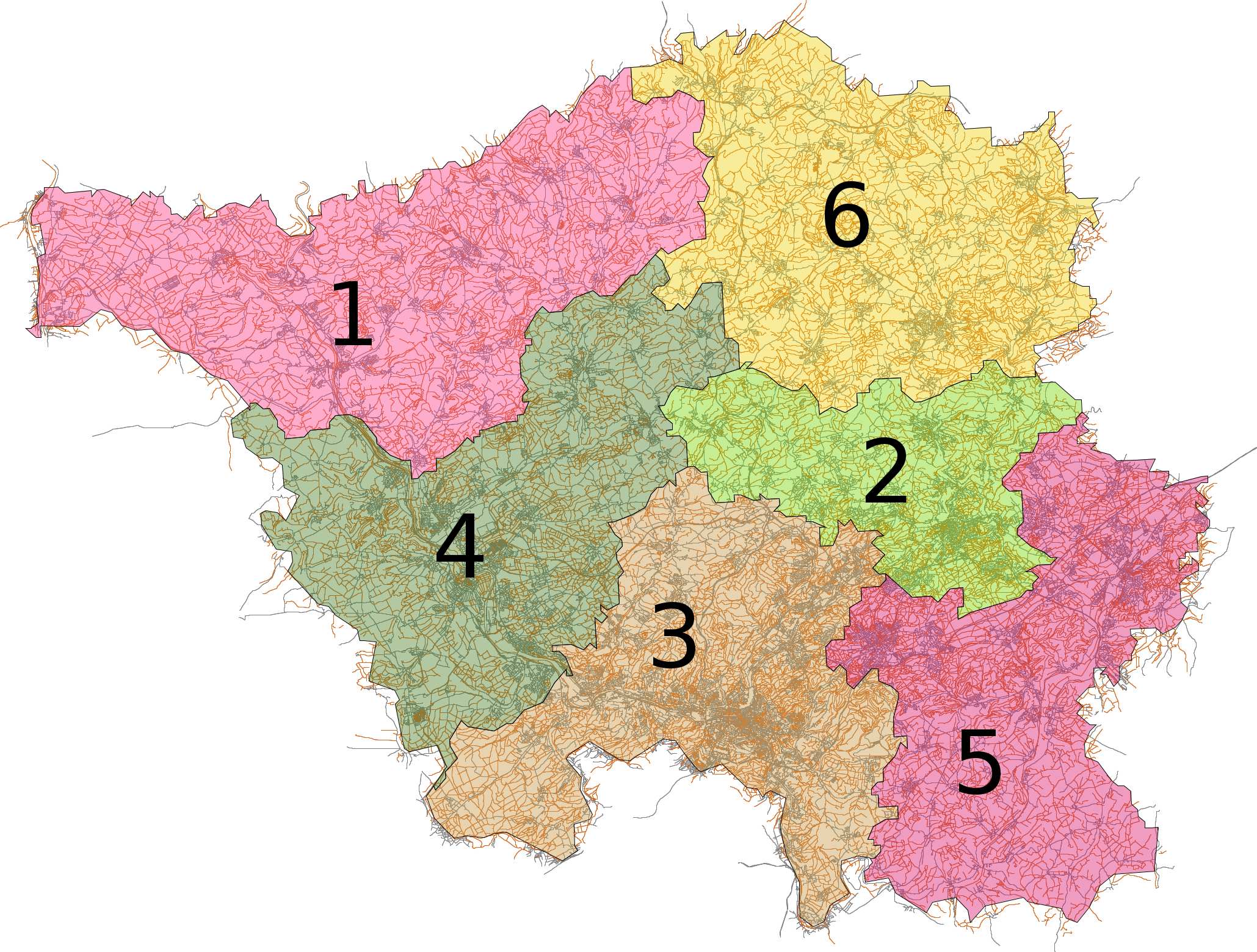
As an example for its quality, the table below shows the results of our population distribution estimation. The algorithm gets the total population of the German federal state Saarland and administrative boundaries of its districts as input. It distributes the population according to the street Voronoi diagram and the edge density clustering. We sum up the streetwise population for each district on the next lower administrative level and compare them to value reported on Wikipedia.
| district | population | ||
|---|---|---|---|
| actual | estimated | relative deviation |
|
| 1 Merzig-Wadern | 103,520 | 96,903 | -7% |
| 2 Neunkirchen | 134,099 | 118,628 | -12% |
| 3 Saarbrücken | 326,638 | 315,866 | -3% |
| 4 Saarlouis | 196,611 | 175,705 | -11% |
| 5 Saarpfalz-Kreis | 144,291 | 157,316 | +9% |
| 6 St. Wendel | 89,128 | 107,452 | +21% |
Quality of the utilization model
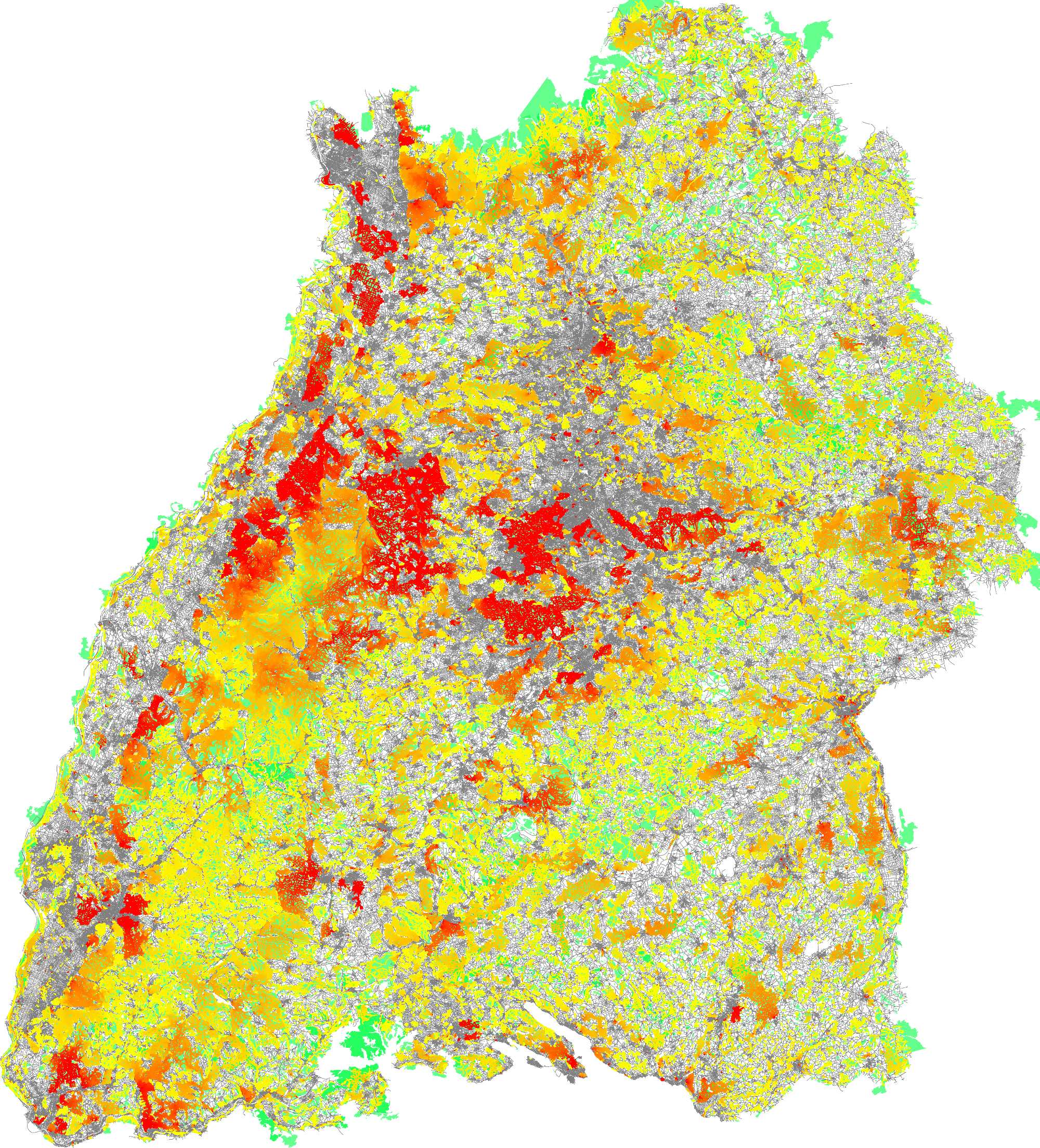
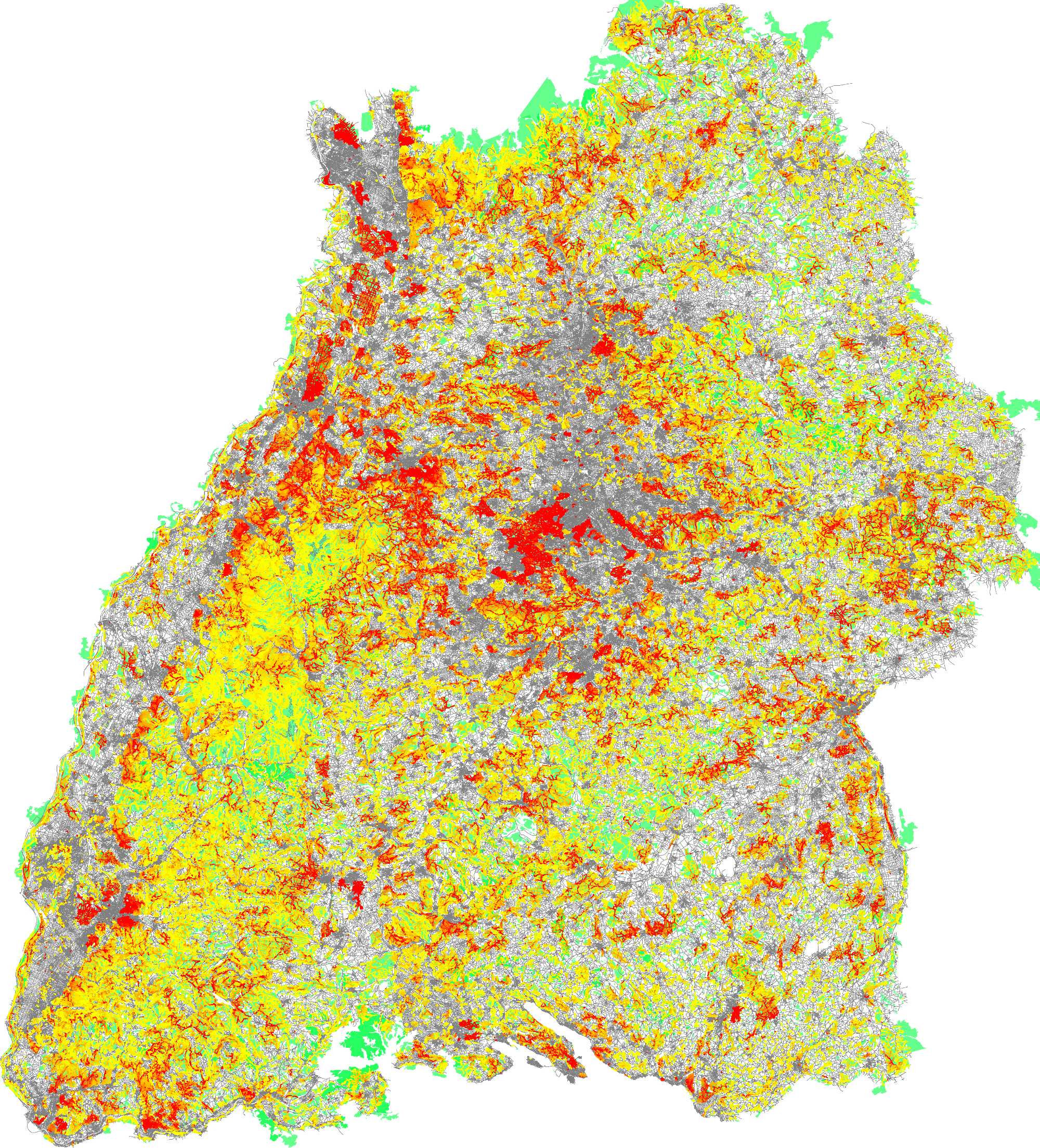
Measuring the quality of our model was quite hard, since there is no ground truth available. OpenStreetMap maintains a huge collections of user-submitted GPS traces. You can get these via the project's main page or excerpts thereof from this page. We filtered this data for traces in the data sets on which we computed our utilization distribution. The following images show the overlaid GPS traces (middle) and the utilization heat maps computed by the flooding approach (left) and the via-edge approach (right) for the Baden-Württemberg data set.

Then we detected the top-50 hot spots of the data by discretizing is to a 1000x1000 grid. After calculating our model, we detected its hot spots in the same way. The following table show the results.
| Graph | Edge Coverage | Hot Spot Detection | |||
|---|---|---|---|---|---|
| OSM | flooding | via-edge | flooding | via-edge | |
| Saarland | 37 | 99 | 100 | 27 | 38 |
| Switzerland | 28 | 97 | 100 | 20 | 24 |
| Baden-Württemberg | 29 | 95 | 100 | 22 | 31 |
| Austria | 22 | 93 | 100 | 18 | 23 |
| Germany | 26 | 91 | 100 | 17 | 24 |
These quantitative results show an advantage for the via-edge approach over the flooding approach. However, that advantage is smaller than one might expect from the visual comparison of the pictures above. This is because the grid discretization and the top-50 approach over-emphasizes the (easy to find) top hot spots, while it does not take the more subtle differences between flooding and via-edge into account. But these regions below the top-50 form the majority of the model.
Downloads
Data sets
Source code
Prerequisities
The steps to reproduce the experiments have been tested on an Ubuntu 13.04 installation. In order to compile and execute the code you need to have GCC, Java 7, Python 2.7.x and some side packages installed. The following should do the trick:
sudo apt-get install build-essentials openjdk-7 python python-numpy
Instructions
After downloading the diverse components, extract the tar balls to some directory.
OSM Parser
Run the parser with this command:
python forestentrydetection.py <OSM_FILE>It will produce the graph files with a label marking nodes inside the forest and forest entries.
Population distribution estimation, forest edge attractiveness.
First, compile the C++ code using the Makefile
cd DEMOGRAPH/
make
The execute the program with the graph from the parser and the population estimate as input.
./demo-graph <GRAPH> <POPULATION>This creates the edge labels file.
Heatmap Server
The Python server can be started
python heatmap_server.py <LABELED_GRAPH>
Background information
This website is built using
About us
The authors of this project are Hannah Bast, Jonas Sternisko and Sabine Storandt. We are researchers at the university of Freiburg, Germany. You can find further information about our work at our group's website. If you have any questions regarding this project, how to reproduce our results or suggestions for improvement, you can find our email addresses there.